Metric Monitoring

Metric monitoring displays metric data of each resource. You can monitor metric values and trends in real time, add desired metrics to a dashboard, create alarm rules, and export monitoring reports. In this way, you can monitor services in real time and perform data correlation analysis.

Procedure

  1. In the navigation pane, choose Monitoring > Metric Monitoring.

  2. Select up to 12 metrics to be monitored.

  3. Set metric parameters according to Table 1, view the metric graphs on the right, and analyze metric data from multiple dimensions.

    Table 1 Metric parameters

    Parameter

    Description

    Time Range

    Time period when metrics are monitored.

    Statistical Cycle

    Interval at which metric data is collected.

    Interpolation mode

    Method used to measure metrics.

    Note

    The number of samples equals to the count of data points.

More Operations

You can also perform the operations described in Table 2.

Table 2 Related operations

Operation

Description

Adding a metric graph to a dashboard

Click Add to Dashboard to add your desired metric graph to a dashboard.

Adding a threshold rule for a metric

After selecting a metric, click Add to Threshold Rule to create a threshold rule for the metric.

Exporting a monitoring report

Click Export Report to export a metric graph as a CSV file to a local PC.

Setting an interpolation mode

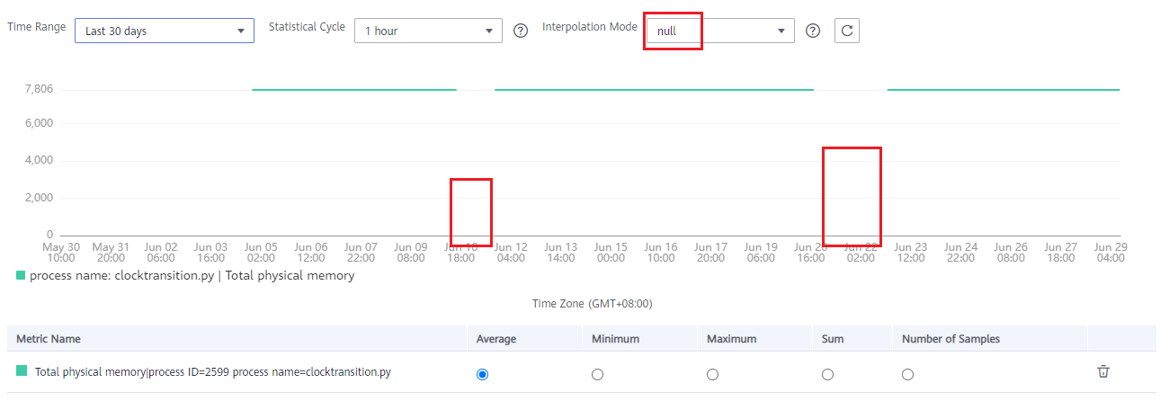
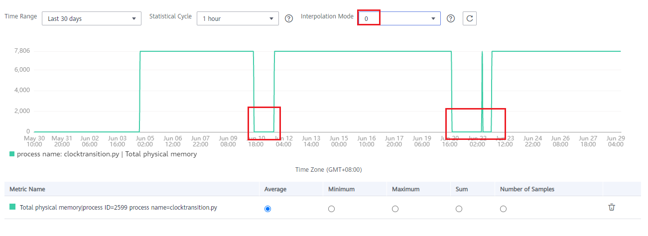
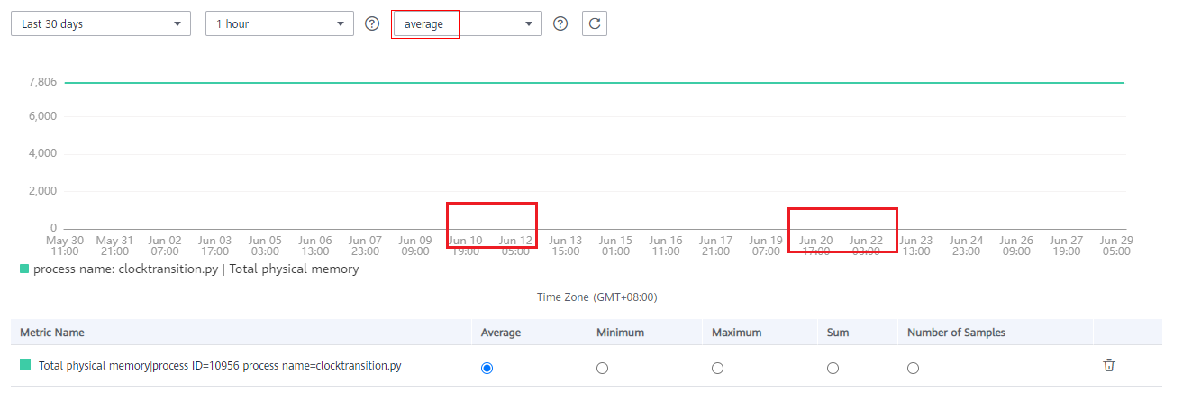
By default, AOM uses null to represent breakpoints in a metric graph, as shown in Figure 1. However, a metric graph with breakpoints is not suitable for reports or presentation. You can replace the missing metric data and avoid breakpoints by setting the value of Interpolation Mode to 0 or average.

The value of Interpolation Mode can be null, 0, or average.

  • null: Breakpoints are represented by null by default, as shown in the following figure.

    **Figure 1** Graph when the value of **Interpolation Mode** is **null**

    Figure 1 Graph when the value of Interpolation Mode is null

  • 0: Breakpoints are represented by 0, as shown in the following figure.

    **Figure 2** Graph when the value of **Interpolation Mode** is **0**

    Figure 2 Graph when the value of Interpolation Mode is 0

  • average: Breakpoints are represented by average values, as shown in the following figure.

    **Figure 3** Graph when the value of **Interpolation Mode** is **average**

    Figure 3 Graph when the value of Interpolation Mode is average

Note

If the value of Interpolation Mode is set to average, breakpoints will be represented by average values. The following describes how to calculate average values.

A metric graph may have multiple breakpoints. When multiple breakpoints exist, values will be interpolated for these breakpoints from left to right. The following uses the first breakpoint in a graph as an example to describe the method of calculating the average value. This method can also be applied to other breakpoints.

  • If the first breakpoint is at the start of a metric graph, the value of the breakpoint is the first valid data from its next point to the right.

    For example, if a metric graph has points a, b, c, d, and e, where a = Null, b = Null, c = Null, d = Null, and e = 5, the value of the first breakpoint (that is, point a) is 5.

  • If the first breakpoint is in the middle of a metric graph, there are the following two scenarios:

    Scenario 1: If the values of the previous and next points of the breakpoint are valid, the value of the breakpoint is the average value of these two points.

    For example, if a metric graph has points a, b, c, d, and e, where a = 1, b = Null, c = 3, d = Null, and e = 5, the value of the first breakpoint (that is, point b) is (a + c)/2 = (1 + 3)/2 = 2.

    Scenario 2: If the value of the previous point of the breakpoint is valid and the value of its next point is null, the value of the breakpoint is the average value of its previous point and the first valid data from its next point to the right.

    For example, if a metric graph has points a, b, c, d, and e, where a = 1, b = Null, c = Null, d = Null, and e = 5, the value of the first breakpoint (that is, point b) is (a + e)/2= (1 + 5)/2 = 3. Because values are interpolated for breakpoints from left to right, the value of the second breakpoint (that is, point c) is (b + e)/2 = (3 + 5)/2 = 4, the value of the third breakpoint (that is, point d) is (c + e)/2 = (4 + 5)/2 = 4.5.

  • If the first breakpoint is at the end of a metric graph, the value of the breakpoint is the value of the previous point.

    For example, if a metric graph has points a, b, c, d, and e, where a = 1, b = 2, c = 3, d = 4, and e = Null, the value of the first breakpoint (that is, point e) is 4.

  • If all points in a metric graph are breakpoints, the values of all these points are still null, even though you set the value of Interpolation Mode to average.

    For example, if a metric graph has points a, b, c, d, and e, where a = Null, b = Null, c = Null, d = Null, and e = Null, the values of all breakpoints are null.